
Abstract
Comparison of the distribution of English surnames in modern England versus former colonies with distinction between the relative rareness of the surname and the overall population of persons using that surname. Geographical surname patterns, Monte Carlo population simulations, and Y-DNA results are considered. Some examples using very early written sources are also used to address the controversy of single versus multiple surname origins in England. A reassessment of the DNA data and conclusions of King and Jobling’s 2009 results is also made.
Introduction
Though most English surnames are rare, most people have populous surnames. “In 1881 for example, 90% of the population of England and Wales had the most populous 4% of surnames; and, in 1998, 80% had the 1% most populous.“12 According to the received wisdom, the most common surnames are multi-origin (i.e. they have a population descended from many distinct medieval origins). Most DNA studies available so far do not discredit that. At the turn of the millennium, however, it was claimed that some early DNA evidence showed that the populous surname Sykes was single-origin.3
More generally, there is much controversy about whether a surname might be single- or plural-origin. The family historian Dr George Redmonds, peering through the mists obscuring medieval origins, has offered guidance: given the almost unlimited choice of a name, the re-use of one would be unlikely, implying surnames with only one origin.4 The geneticist Prof Bryan Sykes, who acknowledged George Redmonds in his seminal Sykes DNA study, accordingly used his data to concur that Sykes is single-origin.3 However, as we shall outline in some detail, if the Sykes name were ascribed only once, there are difficulties in explaining its large population, unless for example we allow that it could have been allocated to a few people, its once being at a single place.
Sykes is believed to have been formed as a locational name, with its first bearers living at a place near some ditches (i.e. sykes). The English surname Plant, also, might have been locational – its dominant family is found first near a newly planted vaccary, meaning a newly founded cattle rearing station. However, for a single beginning, much medieval migration would have been needed between many distantly separated records of the Plant by-name, some of which showed that this surname had already become hereditary in a few different places.
As another relevant view, we could accept a proposition made by the onomastic linguist Dr Richard Coates: a peasant did not normally choose his own surname.5 We can accordingly imagine a scribe who chose to use, in his records of a medieval manorial court’s proceedings, a succinct single name for a small group of men. Such men could have shared local ancestry which would explain why DNA-matching populations are large in some common English surnames. However, this version of events relies not least on a hazy view of a scribe’s predilections.
More traditionally, the belief is that prolific surnames such as Smith have plural origins, which arose in different places. We will assess this quantitatively below, to the extent that we will consider that common and very common surnames, with UK populations over ten thousand or so, need to have had more than one fourteenth-century forefather.
Some geographical evidence
One simple, though indirect, way of assessing whether a surname could have been single-origin is to examine the 1881 geographical distributions of some populous English surnames. This can be done easily using Steve Archer’s Surname Atlas CD.6 Proceeding on the basis of just their 1881 distributions, the top 140 most common UK surnames all appear to be multi-origin in so far as they are all widely spread. The most common, Smith, has an 1881 population of 422,733 which is considerably more than for Metcalf (6,065), Sykes (14,383) or Plant (6,615) for example, which nonetheless are in the top 750 of most common UK surnames in the 1881 UK Census. George Redmonds has claimed that the surname Metcalf is single-origin; but, Figure 1(a) lends this little support. A little more convincingly, there appears to be a possible dispersal mostly from a single source for the surnames Sykes (Figure 1(b)) and Plant (Figure 1(c)). We give fuller details elsewhere.7
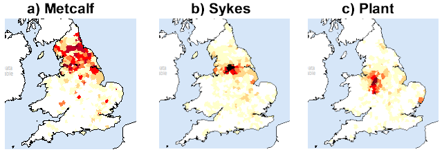
Fig. 1: The 1881 distributions in England and Wales of: (a) Metcalf; (b) Sykes; and, (c) Plant
Figure 2 displays the four most common single-origin contenders, based on their 1881 distributions, in each of six English counties. These counties are displayed in the order of decreasing Industrial Age growth, during 1761 to 1841.8 There are large single-origin contenders in West Yorkshire and Lancashire on the left; and, on the right, less populous contenders in Shropshire and Wiltshire. However, overall population growth in a region between 1761 and 1841 does not explain, for the central two counties, why the most populous single-origin contenders in Cheshire have lower populations than those in Staffordshire.
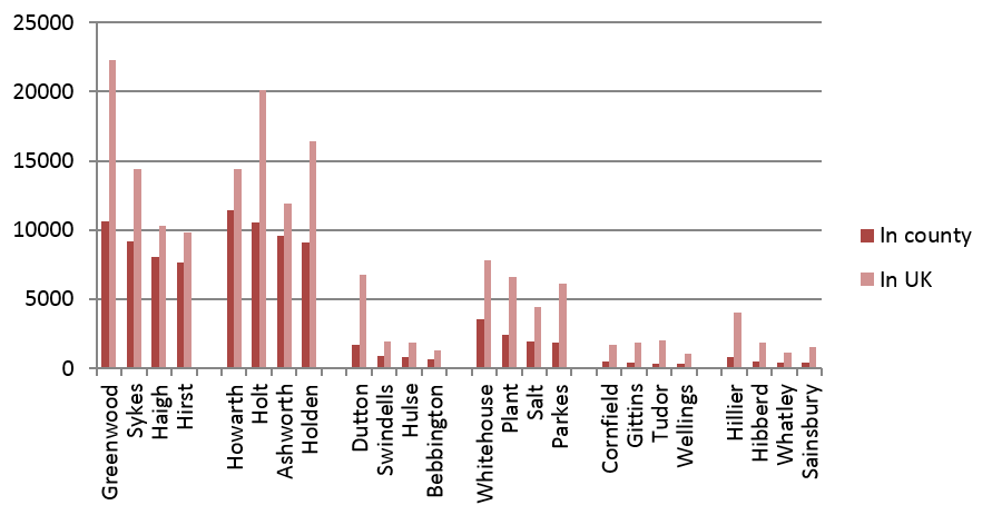
Fig. 2: Populations in the UK in 1881 of the four most-populous single-ancestor contenders in West Yorkshire, Lancashire, Cheshire, Staffordshire, Shropshire, and Wiltshire
Some computer simulations of single-origin surname growth
Figure 3 shows the histogram of single family size by 1881, computed from a type of computer model called a Monte Carlo simulation in which differences in family size occur as a result of pure chance without any additional distinguishing factors. Further details of our computer simulations are given in Appendix 1. For Figure 3, 1,000,000 simulations are computed for an English family starting in 1311 and, by 1881, the male-line family dies out in 92.5% of cases; whereas, in the largest outcome, it grows purely by chance to 730 active males by 1881, at the barely discernible tail end in Figure 3. Only reproductively active males are considered; namely the ones who usually pass on the surname, together with their Y-chromosome, to fertile sons who in turn have sons of their own. A multiplier of around four to six can be applied to the number of reproductively-active males to give the predicted population of the whole descent family population of a single-origin surname. We can hence note that there is a prediction of around 4,000 for the largest single-origin family size by 1881 – this falls short of the observed values for the top 750 English surnames which, as we have already indicated, have UK populations over 6,000 in 1881. Before jumping to a conclusion that these surnames must be multi-origin, we have first tried feeding further factors into our computer simulations to see if we can increase the sizes of the largest predicted single-origin descent families.
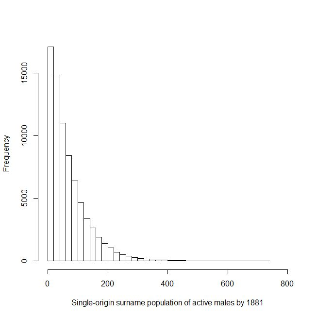
Fig. 3: Computed chance (frequency out of 1,000,000 in 1311) of a single-origin family growing to various active-male population sizes by 1881
As an extension to our basic model, Table 1 displays the largest single-origin families predicted by 1881, for each of six historic (pre-1965) counties. The numbers represent reproductively active males. They display the largest reproductively-active male populations, arising by random chance, given a local environment of particular growth conditions. Instead of the all-England growth parameters of the basic model, we have here used ones derived from published county-wide population data.
Yorkshire
Lancashire
Cheshire
Staffordshire
Shropshire
Wiltshire
831
658
577
1,246
332
229
The largest families, shown in Table 1, arise as very rare “one in a million” events. They best serve to illustrate the differences between counties.
Figure 3 displays instead average growth curves, for the largest 0.1% of initial families. Since most families die out, these curves apply to about the largest 1.3% of surviving families. It can be seen that the fortuitously large families are predicted to grow in Cheshire, Yorkshire and Lancashire to around the same size as in the basic model for all England. There are some marked differences however. Predicted large families grow much larger for Staffordshire and much less for Shropshire and Wiltshire. Such differences are broadly in line with the observed evidence outlined in Figure 2, except that excessively large single-origin contender surnames were identified in Figure 2 for West Yorkshire and Lancashire. Our computer simulations at least illustrate that, neglecting possible net migrations between counties, different growth conditions in different parts of England can have significant effects on the predicted sizes of the largest descent families. We might add that the excessively large single-origin contender surnames in West Yorkshire and SE Lancashire might well have arisen in long-standing wool-wealthy regions, where there could have been economically favourable growth conditions that were not typical of these two counties as a whole.
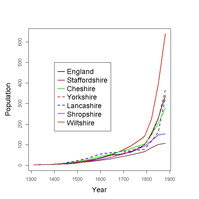
Fig. 4: Growth of the largest 0.1% of the initial families under different county-wide growth conditions
Additional factors are particularly needed if we are to explain the claimed single-family size for the populous surname Sykes. Geographical distribution maps in 1881 suggest that Sykes is the second largest “single-origin contender” surname in West Yorkshire (Figure 2). To explain the exceptionally large size of this “contender” surname, we might consider that the general growth conditions in pockets of West Yorkshire were as favourable as those of Staffordshire. Adopting a different hypothesis, George Redmonds and Bryan Sykes have suggested that the apparently large size of the Sykes family might be due to a genetic advantage being passed down its male line.4 We will hence consider the possibility of a still further enhancement of the growth rates beyond those of Staffordshire.
The green lines in Figure 5 correspond to simulations with an enhancement of 6% over the overall Staffordshire growth rates. We also consider a family’s supposed resilience to the mid fourteenth-century Black Death. This hypothetical resilience (blue lines) has little effect on a large descent family’s predicted population by 1881 (Figure 5(b)) whereas the persistent 6% enhancement from 1311 to 1881 (green lines) is much more effective.
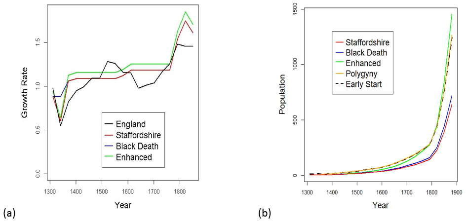
Fig. 5: Growth rates (a) for England and Staffordshire and (b) population growth curves for fortuitous families
Figure 5(b) shows similar effects from two other favourable factors: fourteenth-century polygyny (yellow line) or an early start to the surname (broken black line). These can similarly increase the growth of a family’s population substantially. In the polygyny model, the extra growth is achieved by either the first male of the family having seven mistresses or he and his sons each having three. The polygyny model requires that all of the resulting offspring carry the same surname, suggesting that we should perhaps substitute the idea of successive wives for mistresses. Alternatively, in the early-start model, much the same growth is achieved by there being twelve active males in a single family bearing a shared surname by 1311. This could arise by a surname having originated ten generations (around three centuries) earlier; or, by that many related men being ascribed the same surname in 1311. For example, these twelve male-line related men might have acquired the same surname by living near the same system of ditches (Sykes) or a medieval fertile enclosure (Plant).
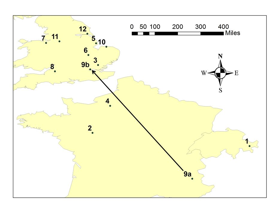
Fig. 6: Some medieval records for Plant-like names
(1) 1139-1798 Seat of the noble Planta family in the Upper Engadine (2) 1202 Lands at Chinon and Loudun of Emeric de la Planta alias de Plant’ (3) 1262 First known evidence of the name in England; spelled Plaunte (4) 1273 Three Rouen merchants called de la Plaunt and Plaunt (5) 1279 At Burgh-le-Marsh near Bolingbroke, the name Plante is indicated to have been hereditary for 3 generations (6) 1282 The name form de Plantes in Huntingdonshire (7) 1301 First evidence of the Plant name local to the subsequent main homeland of the surname (8) ca.1280-ca.1360 Records of Plonte name at Bath, explicitly hereditary by 1328 (9) 1350 London priest Henry Plante of Risole: (9a) is Risoul; (9b) is London (10) 1352 James Plant carried away goods from recently lost Warren lands in Norfolk (11) 1360 onwards Several records of Plonte or Plont in the subsequent main Plant homeland (12) 1379 A gardener called Plant See http://www.plant-fhg.org.uk/origins.html#13c for a fuller list and details.
Some computer simulations for plural-origin surnames
Detailed data for the medieval origins of surnames is still difficult to assemble, even with the advent of some historic sources that are more readily available on the internet. We have gathered such data for the Plant surname, which is discussed more fully in Appendix 2. Plant is the second most populous single-origin contender surname for Staffordshire (Figure 2). However, our computer simulations and DNA evidence, along with medieval records, suggest that this surname is plural-origin, albeit with one dominant family that has grown abnormally. As Figure 6 illustrates, this moderately common English surname, with a living UK population around twelve thousand, appears to have more than one origin, unless we imagine a single origin with a surprising degree of medieval migration.
We have hence extended our computer simulations to the modern day and considered the possibility of there being several surviving separate-origin descent families within a single surname.
Figure 7 shows some computer simulation results for the example of two thousand reproductively-active men, corresponding to a moderately-common English surname of around eight to twelve thousand living people in the UK.
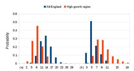
Fig. 7: Predicted probabilities
Predicted probabilities of (a) the number of separate-origin male-line families in a surname with 2,000 reproductively-active males; and, (b) largest family in hundreds of reproductively-active males.
Starting with Figure 7(a), this displays the predicted chances of there being different numbers of surviving separate-origin families in a moderately-common surname’s living population. The tallest blue bars in Figure 7(a) illustrate that we can expect around thirteen separate-origin descent families in a surname that experiences the general population growth rates of England; there is some spread of uncertainty, due to random fortuity, as represented by the spread of the bars. Rather fewer descent families (orange bars in Figure 7(a)), with a spread around seven, are expected for a surname of this size, if its families are in a geographical region such as Staffordshire where the general population data indicate average growth rates that have been relatively high.
Moving on to Figure 7(b), this shows that the largest UK descent family in a moderately-common surname is likely to have around five hundred reproductively-active men, if it experiences only the average growth conditions in England. This corresponds to the tallest blue bar. However, for the high-growth region of the orange bars, a single-origin descent family might grow as large as fifteen hundred or more such men, though the shorter bars indicate that this has a lower chance of arising. In other words, Figure 7(b) predicts that the size of the largest descent family in a moderately-common English surname will generally be below three quarters of the surname’s population. This corresponds to a DNA matching fraction of below 0.45, provided that we assume a non paternity event (NPE) rate of 2% per generation. If the NPE rate were assumed to be lower, the predicted matching limit would be lowered less from 0.75.
We have also generalised the simulations to English surnames with a larger range of sizes. Figure 8 shows that the predicted UK population of a single-origin descent family can extend from a few to around ten thousand (as shown for just one descent family at the extreme right of the figure). With a hundred descent families in the surname, its predicted UK population can readily extend to over a hundred thousand.
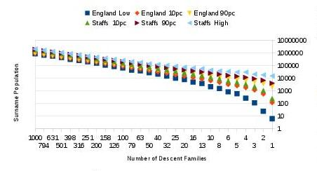
Fig. 8: Predicted whole surname populations in the UK
Predicted whole surname populations in the UK for different numbers of descent families in the surname. There is an 80% chance that the surname’s population will fall between the computed 10th percentile (10pc) and 90th percentile (90pc) in the probability distribution of the surname’s predicted size. The graph also displays the lowest predicted surname size with the all-England growth conditions (dark blue squares) and the highest predicted surname size in the high-growth Staffordshire conditions (light blue triangles).
Some relevant DNA evidence
Turning to some observed data, for comparison with our simulation results, the UK populations of some real surnames are represented by the blue diamonds in Figure 9. These populations range from 148 (Feakins) to 775,645 (Smith). Most of the surnames in Figure 9 have UK populations below ten thousand. It is hence to be expected that some of the smaller surnames could be single-origin and contain just one small or moderately-sized descent family. On the other hand, the whole population of the very common surname King, for example, exceeds this single-family limit, implying that it should have many other separate-origin descent families besides its largest.
Mostly, this is confirmed by the evidence in Figure 9. This Figure includes an indication of the size of each surname’s largest biological cluster, which can be taken to represent a descent family that contributes towards the surname’s whole living population. Most of the underlying DNA data, for the red squares, comes from a study by the geneticists Dr Turi King and Prof Mark Jobling (K&J) though they themselves did not use their data in this way.9 Many of the red squares for the smallest surnames leave little room for other small families besides the largest, especially after allowing for the effects of non paternity events (NPEs). This is less true for some larger surnames, such as Jefferson. For King, its red square suggests that it has a largest biological descent family of around ten thousand, leaving room for many other descent families in its UK population which exceeds a hundred thousand. However, the red square for Smith suggests a single family size of around a hundred thousand, far exceeding our predicted limit. Even so, room still remains for many other families. We will proceed to offer an explanation for the Smiths’ high red square and the absence of an observed matching cluster for Bray.
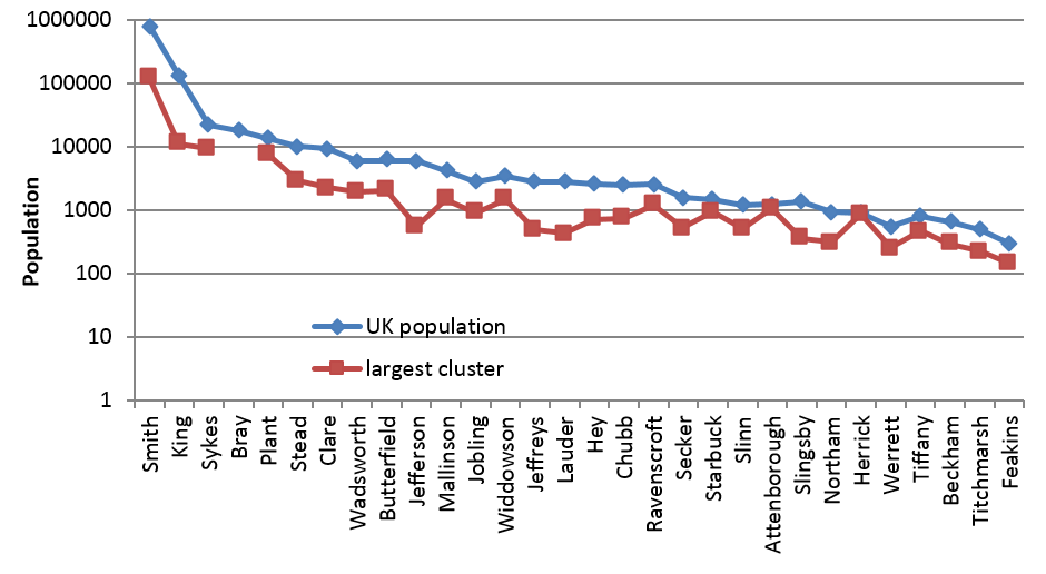
Fig. 9: Largest cluster populations in some UK surname populations
It is important to bear in mind some practicalities of the DNA determinations.
The red square for the largest descent family, in the case of King or Smith, is derived from a relatively small DNA cluster: a cluster of two in a sample of 24 in the case of King; and, a cluster of nine for Smith. Small clusters are sensitive to statistical bias and sampling error. For Smith, its observed 15.5% DNA cluster might arise from the limited DNA resolution used by K&J, which may not have distinguished adequately between separate medieval families for this surname. It is hence just dubious speculation that a particular family of smiths might have had a very early genesis followed by an anomalously high male-line growth. That would be at odds with the predictions of our computer model simulations, at least with its simplest assumptions.
Another practicality arises in connection with the gap in Figure 9 for the fourth surname, Bray. It indicates that K&J found no observed DNA cluster in their sample of 29 men. This observation implies a limit of 7% on the fraction that would match hypothetically in a larger random sample of this surname’s UK population. This is quite similar to the 9% fraction found for a larger sample of the smaller surname Jefferson.
We should add that it is not generally reported whether hobbyist’s DNA samples are biased to over-represent particular families. Our analyses assume a random sample of the surname’s whole population in a region; we here consider in particular men living in the UK. The K&J data were obtained from a truly random sample, but other surname data are almost never obtained this way. Instead, to use the statistical term, the data are obtained “haphazardly”. This does not cause a serious problem provided that data values are obtained independently of each other. However, one-name researchers often target particular families in a surname, or sometimes deliberately target at least two in each genealogical family, regardless of each family’s size. This can produce a statistical bias that is significantly misleading for our purposes.
The observed largest DNA descent clusters (red squares) in Figure 9, for moderately-common surnames, largely confirm our computer model prediction that English surnames of a “moderately-common size” can be expected to have DNA matching values below 0.45. For Sykes, Bray, Plant, Stead, Clare, Wadsworth, Butterfield and Jefferson, the observed fractions are 0.44, <0.07, 0.50, 0.28, 0.24, 0.33, 0.33 and 0.09 respectively. For the high value for Plant, it should be added that there is a 0.12 standard error of statistical uncertainty arising from the limited sample size.10 It would seem that all of these surnames are plural origin albeit that some evidently have a dominant family that accounts for a large fraction, perhaps around three quarters, of this surname’s whole UK population.
The anomalous K&J result for Smith
As already mentioned, at face value K&J’s DNA result for Smith in Figure 9 suggests a descent family size of around a hundred thousand in the UK, far exceeding our predicted limit of around ten thousand. Rather than immediately concluding that our computer simulations fall short, it is relevant to re-assess K&J’s DNA data and in particular their control sample.
Though one might expect, purely as a statistical coincidence, an exactly matching pair of Y-STR haplotypes somewhere within K&J’s control sample, there is much less chance of there being a second pair at the same place. In fact, the control sample contains a significant cluster of three exactly matching pairs immediately neighbouring one another. We will call this the TPCC (three pairs cluster core). This is not mentioned by K&J, who instead quoted an h-statistic indicating that neither their control nor the Smith sample displayed much clustering.
When a single family dominates a given surname, it is relatively straightforward to identify and assess a single DNA descent cluster; but, the apparent evidence can be more confusing in the case of many descent families in a very common or prolific English surname. For these, even an abnormally large descent family represents only a small fraction of the surname’s whole population. In particular, a small apparent cluster for a surname might readily be confused with the aforementioned TPCC.
The relevant K&J results are outlined in Table 2. For Smith, an exactly matching triplet is found at a single haplotype value. This is significant in that not only is there a matching pair for Smith but there is also a third person in the Smith sample who matches exactly. Moreover, this Smith triplet haplotype also matches the TPCC haplotypes in the control sample. In so far as the Y-STR markers used by K&J overlap with the more commonly used markers of commercial testing companies such as FTDNA, this Smith triplet corresponds to WAMH1 (Western Atlantic Modal Haplotype 1), which is the most common Y-STR signature found in the general population throughout Europe and North America.1112 Similarly, the three haplotypes of the TPCC correspond to the WAMH1, WAMH4 and an immediately adjacent haplotype. We can hence identify the observed triplet for Smith with the most common haplotype signatures in the general population of Western Europe and, more particularly, the TPCC in K&J’s control sample for England. In other words, K&J’s “true cluster” for Smith appears to be a manifestation of a convergence cluster for the general population and hence it cannot be taken as a large descent family that has grown abnormally since the times when the Smith surname formed.
At the root of the confusion are some arbitrary rules used by K&J to identify a “true cluster” in their data. For the Y-DNA haplogroup R1b1 (and similarly for the haplogroup I), they adopted a rule that a “true cluster” had to have at its core a matching triplet at a single haplotype. They hence reported that there was no true descent cluster in their control sample, despite the TPCC, but a cluster of nine near matches for Smith surrounding the exactly matching triplet. We consider that their rather arbitrary rules for “true clusters” fall down in this case. Indeed, K&J themselves tacitly seem to acknowledge this elsewhere in their paper,9 by simply stating that they found no significant evidence for a descent family size larger than ten thousand for any of the surnames they examined.
The seventeen Y-STR markers used by K&J and their values for the matches found in their Smith sample and their control sample.
Maker
Smith (41 42 43)
Control Brown Bryson
Control Badge Evans
Control Lawson Snow
ISOGG WAMH 1
ISOGG WAMH 2
ISOGG WAMH 3
ISOGG WAMH 4
FTDNA Super WAMH
DYS436
12
12
12
12
12
DYS437
15
15
15
15
15
DYS438
12
12
12
12
12
DYS434
11
11
11
11
DYS435
11
11
11
11
DYS439
12
12
12
12
12
12
11
12
12
DYS389I
13
13
13
13
13
13
13
13
13
DYS389II-I
16
16
16
16
16
16
16
16
16
DYS461
12
12
12
12
DYS462
11
11
11
11
DYS460
11
11
11
11
11
DYS391
11
11
12
11
11
10
11
11
11
DYS390
23
23
24
24
23
24
24
24
24
DYS393
13
13
13
13
13
13
13
13
13
DYS392
13
13
13
13
13
13
13
13
13
DYS388
12
12
12
12
12
12
12
12
12
DYS19
14
14
14
14
14
14
14
14
14
Haplogroup
R1b1
R1b1
R1b1
R1b1
Figure 10 compares the MEGA6 diagrams13 for Smith and the control sample. It illustrates that nothing by way of a “true cluster” of nine stands out for Smith. Though the triplet (Sm42, Sm43, Sm41) of exact matches can be discerned for Smith, this does not seem obviously to form a basis for a cluster of nine – it does not appear to be significantly different from a general background diffuse cluster to be found around the genetically adjacent matching pairs (TPCC) in their control sample of many different surnames. The three pairs of the TPCC are Brown-Bryson, Badge-Evans, and Lawson-Snow; though it is not obvious in this MEGA6 diagram that these three pairs are genetic neighbours.
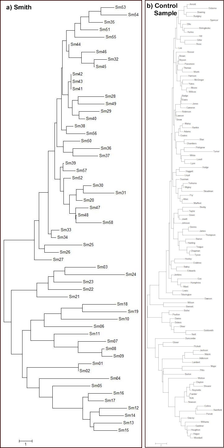
Fig. 10: MEGA6 Diagrams
MEGA6 diagrams of K&J’s 17 marker Y-STR UK data for (a) Smith and (b) their control sample.
Emigration
We can accordingly surmise that the available data does not discredit our computer simulations for common English surnames. We have hence proceeded to extend our computer model to include emigration. For this, we have derived, from published data, some historical rates of emigration assuming that it occurs randomly. However, it seems that there might have been a small non-random component to the way in which some surnames migrate. Non-random emigration could have arisen, for example, as follows. A surname’s largest family in the UK might have grown abnormally and we can conjecture that this would have placed pressure on inherited land. Hence smaller, widely-spread English families might be expected to have had lower historical rates of migration than a large family experiencing land shortages.
DNA evidence suggests that there could have been non-random emigration, with a difference for small and large families, for the illustrative example of the plural-origin surname Plant. For this surname, the observed DNA matching fraction is 0.50 for a sample of sixteen men living in the UK, as against 0.71 for twenty-one men living overseas.10 Though this noticeable difference is not statistically significant at the 95% confidence level, it does not rule out non-random emigration. There could be several small descent families, lowering the DNA matching fraction in the UK. It could then be that the dominant descent family has emigrated disproportionately more, leading to a higher DNA matching fraction in the diaspora. Such non-random migration might show up in other ways.
For a wide range of surname sizes, Figure 11 presents some results from our computer simulations, which here assume purely random emigration. The simulated populations (grey circles) show that the overseas populations of the surnames increase roughly in line with their UK population. The superimposed coloured circles are for a few moderately-common real surnames (UK populations around 10,000). These surnames tend to lie towards the lower edge of the grey circles, indicating relatively low emigration rates. On the other hand, the triangles are for very common surnames (UK population around 100,000) which tend to reach more often towards the upper edge of the grey circles. This observed trend has been found for many real surnames. This trend might relate partly to our aforementioned comments on non-random emigration.
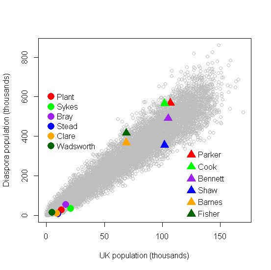
Fig. 11: Simulated relationship between UK and diaspora populations, with some data for real surnames superimposed.
Acknowledgements
This article was peer reviewed with 3 commentaries.Appendix 1
Further details of our Computer Simulations
In this appendix, we describe the assumptions made in the Monte Carlo simulation model used to explore the probabilities of outcomes associated with population growth. The model keeps track of reproducing males. It assumes a 1:1 sex ratio and considers only males that survive to procreate in the next generation. We assume that approximately one third to one half of the total males population are reproductively active, the remainder being either too young or too old. The number of male children born to each father and surviving to adulthood is assumed to be a random variable drawn from a Poisson distribution. For purposes of brevity, we will not continue in the description of the model to specify that we only include male offspring who survive into adulthood; this will be implicit in the discussion. The Poisson distribution is characterized by a single parameter: the mean (in our case, the mean number of surviving male children in each family). This number is computed according to the theory of branching processes as described by Pinsky and Karlin14 from the rate of population change in England in each generation. Population data were taken from Hatcher and Bailey15 for the period from 1311 to 1541, and from Wrigley and Schofield16 for the subsequent period. Medieval county-level population data are taken from Broadberry et al17 and county population data for the period after 1800 are taken from census records.
Our model computes the number of male descendants of each progenitor by generating a random variable each generation representing the number of male offspring from each descendant in the current generation. This describes a type of branching process called a Galton-Watson process. An important property of such models is that the individuals do not interact with each other. That is, each individual in each generation procreates in isolation from the others; there is no competition for resources. Again, although this may not reflect the conditions of the real world, it does produce a sufficiently accurate simulation, because the effects of the competition are reflected in the overall population growth rate values.
The population of England in 1311 is conservatively estimated to have been approximately two to three million, implying a reproducing male population of approximately five hundred thousand. The generation time is a key variable in the simulation. Although the human generation time is often taken to be about 25 years, recent research suggests that it is longer, possibly as long as 35 years. We use a generation time of 30 years. This is based on the assumption that the generation time can be taken to be the mean maternal age at birth. Wrigley and Schofield show that in England this age had a consistent value of about 31 to 32 years from the sixteenth through the nineteenth century. We took the value of 30 as a round number that reflects a possibly shorter generation time during earlier centuries.
The county growth rates used for Figure 4 were derived from county-wide population data and are shown in Figure 5. Further details concerning the simulations are given elsewhere.7 10
Appendix 2
Application to the meaning of Plant
There was a gardener with the Plant by-name, as an isolated instance in East Yorkshire in 1377.4 It would be an example of an “availability error”, however, to envisage plants only in modern gardens. The Plant by-name sometimes has a locative form, as indicated by the prefix de la for example: for a landholder Eimeric de la Planta in Anjou in 1202; for three Rouen merchants called de la Plaunt and Plaunt in 1273; and, for Henry de Plantes in Huntingdonshire in 1282.7 18 Identifying specific places for the locative origins of these name forms is not without problems, though there are the place names Le Plantis in Normandy and La Planteland in the Welsh Marches.19 20 In French, plante can mean a vegetable bed, perhaps giving rise to minor place names. In Welsh, the word’s senses extend however to procreation and the offspring of animals and humans.18 Such extended meaning is apparent also in the context of medieval Latin and Middle English, for which the nutritive, augmentative and generative powers of the medieval plant soul were believed to exist in vegetables, animals, humans and even minerals.21
For the main Plant family, we might consider that, before the industrial sense, the Plant name could have been associated with all of the medieval plant powers of feed, growth and breeding at the Plants’ earliest known location in their main homeland (item 11 in Figure 6). This was at the Black Prince’s vaccary (cattle station) at Midgeley on the Cheshire-Staffordshire border where, in 1373, Thomas Plontt had failed to pay the fine for pasturing a bullock.22 When the Black Prince’s administrators at the Macclesfield Court ascribed the Plants a surname, they might have had the Midgeley “plant” in mind. Some such a locative origin is accordingly possible for the main Plant family, though other possible meanings exist.
Among the various proposals for the origin of the Plant surname, two of the published claims have since suffered from conflicting evidence. First, it was considered in the mid twentieth century that the Plants were multi-origin gardeners;23 but, now, nearly all newly discovered occupations for the early Plants disconfirm this.24 Secondly, our latest Y-DNA results for a better-accredited male-line Plantagenet descendant do not ratify a nineteenth-century claim that the Plants were the Plantagenets’ illegitimate descendants.25 There are also two early twentieth-century claims: Plant meant a `young offspring’ or it was locative.26 These two meanings can be related to our modeling of a large family size.
For the dominant Plant family, the sense `many offspring’ is compatible with our early polygyny model. Instead, a locative origin is compatible with our early start model, since we can conjecture for example that there was a pre-existing family at the location before the formation of the surname. Either model is compatible with the documentary evidence, such as that several Plants have been found in the earliest local pannage (animal pasturing) lists, for which evidence has survived for the main Plant homeland beginning in the 1360s.22 Both models (yellow and broken black lines in Figure 5(b)) allow for the possibility that all of the Plants found in the early Macclesfield Court Rolls of east Cheshire could have belonged to a single family.
Other evidence suggests that there were other less-prolific origins to this surname in other places. For example, the DNA evidence shows that there is a genetically distinct Plante family in Canada, evidently from France and spread into the USA. There is also an indication of a relatively small separate-origin Plant family from SE Lincolnshire in England (cf. item 5 of Figure 6).7 10
References
- Tucker DK. (2007). Surname distribution prints from the GB 1998 Electoral Roll compared with those from other surname distributions, Nomina, 30, pp. 5-22.
http://www.snsbi.org.uk/Nomina.html - Tucker DK. (2008). Reaney and Wilson Redux: An Analysis and Comparison with Major English Surname Data Sets, Nomina, 31, pp. 5-44.
- Sykes B, Irven C. (2000). Surnames and the Y Chromosome. The American Journal of Human Genetics, 66, 4, 1417-1419. doi:10.1086/302850.
http://dx.doi.org/10.1086/302850 - Redmonds G, King T, Hey D. (2011) Surnames, DNA, & Family History, Oxford University Press.
http://www.amazon.com/Surnames-Family-History-George-Redmonds/dp/0199582645/ - Coates R. (2012). private communication with author.
- Archer S. (2003). Surname Atlas CD [software].
http://www.archersoftware.co.uk/satlas01.htm - Plant JS, Plant RE. (2014). Getting the most from a surname study: semantics, DNA and computer modeling (third edition). Guild of One Name Studies.
http://cogprints.org/9191/ - The Cambridge Group for the History of Population and Social Structure. (2011). Department of Geography and Faculty of History, University of Cambridge.
http://www.hpss.geog.cam.ac.uk/research/projects/occupations/englandwales1379-1911/figure2/figure2b.html - King TE, Jobling MA. (2009). Founders, Drift, and Infidelity: The Relationship between Y Chromosome Diversity and Patrilineal Surnames. Molecular Biology and Evolution, 26, 5, 1093-1102. doi:10.1093/molbev/msp022.
http://dx.doi.org/10.1093/molbev/msp022 - Plant JS, Plant RE. (2014). English Surnames: DNA, plural origins and emigration. Guild of One Name Studies.
http://cogprints.org/9748/ - ISOGG. (2014, Oct 12). Western Atlantic Modal Haplotype.
http://www.isogg.org/wiki/Western_Atlantic_Modal_Haplotype - Athey W. (n.d.). The Western Atlantic Modal Haplotype (WAMH).
http://www.hprg.com/R1b/page2.html - Tamura K, Stecher G, Peterson D, Filipski A, and Kumar S (2013) MEGA6: Molecular Evolutionary Genetics Analysis Version 6.0. Molecular Biology and Evolution 30: 2725-2729.
http://www.megasoftware.net - Pinsky MA, Karlin, S. (2010). An Introduction to Stochastic Modeling. Academic Press.
http://www.amazon.com/Introduction-Stochastic-Modeling-Fourth/dp/0123814162/ - Hatcher J, Bailey M. (2001). Modelling the Middle Ages: The History and Theory of England's Economic Development (Oxford Ethics Series). Oxford University Press.
http://www.amazon.com/Modelling-Middle-Ages-Englands-Development/dp/019924412X/ - Wrigley, EA and Schofield, RS, The Population History of England 1541-1871: A Reconstruction. Oxford University Press. 1981.
http://www.amazon.com/Population-History-England-1541-1871-Cambridge/dp/0521356881 - Broadberry S, Campbell BMS, van Leeuwen B. (2011). English medieval population: reconciling time series and cross sectional evidence.
http://www2.warwick.ac.uk/fac/soc/economics/news_events/conferences/venice3/programme/english_medieval_population.pdf - Plant JS. (2005). Modern methods and a controversial surname: Plant, Nomina, 28, pp. 115-33.
http://cogprints.org/5985/ - Boynton GR. (2003). Calendar of Patent Rolls, 1310 Oct 10 Carmyle. University of Iowa.
http://sdrc.lib.uiowa.edu/patentrolls/e2v1/body/Edward2vol1page0313.pdf - Boynton GR. (2003). Calendar of Patent Rolls, 1311 March 7 Berwick-on-Tweed. University of Iowa.
http://sdrc.lib.uiowa.edu/patentrolls/e2v1/body/Edward2vol1page0366.pdf - McKeon CK. (1948). A Study of the Summa Philosophiae of the Pseudo-Grosseteste. Columbia University Press.
http://www.amazon.com/Study-Summa-Philosophiae-Pseudo-Grosseteste/dp/1258636859/ - Plant JS. (2012). Earliest evidence for the Plontt/Plant name in Macclesfield Court Records.
http://www.plant-fhg.org.uk/EarlyPlontsMacclesfield.pdf - Reaney PH. (1958). Dictionary of British Surnames. Routledge & Keepag Paul.
http://www.amazon.com/Dictionary-British-Surnames-P-Reaney/dp/0710081065/ - Plant JS, Plant RE. (2012). The Plant Controversy. Journal of One Name Studies, 11(2), pp. 8-9.
http://www.plant-fhg.org.uk/vol11-2_ThePlantControversy.pdf - Plant JS, Plant RE. (2010). Understanding the royal name Plantagenet - How DNA helps. Journal of One Name Studies, 10(8), pp. 14-15.
http://www.plant-fhg.org.uk/vol10-8_RoyalNamePlantagenet.pdf - Weekly E. (1916). Surnames. New York. p. 185.
http://www.amazon.com/Surnames-Ernest-Weekley/dp/B00AI82YGM
Leave a Comment
You must be logged in to post a comment.